45 how to show alternate data labels in excel

› sort-by-color-in-excelSort by color in Excel (Examples) | How to Sort data with Color? In Excel, there are two ways to sort any data by Color. Firstly, we can sort the data by color through filters. For this, apply the filter selecting an option from the Data menu tab and then select the Sort by cell color or font color from the drop-down option. And other ways is sorting the data using the Sort option available in the Data menu tab. How To Add Axis Labels In Excel [Step-By-Step Tutorial] First off, you have to click the chart and click the plus (+) icon on the upper-right side. Then, check the tickbox for 'Axis Titles'. If you would only like to add a title/label for one axis (horizontal or vertical), click the right arrow beside 'Axis Titles' and select which axis you would like to add a title/label.

Add or remove data labels in a chart - Microsoft Support On the Design tab, in the Chart Layouts group, click Add Chart Element, choose Data Labels, and then click None. Click a data label one time to select all data labels in a data series or two times to select just one data label that you want to delete, and then press DELETE. Right-click a data label, and then click Delete.

How to show alternate data labels in excel

support.microsoft.com › en-us › officeDesign the layout and format of a PivotTable In a PivotTable that is based on data in an Excel worksheet or external data from a non-OLAP source data, you may want to add the same field more than once to the Values area so that you can display different calculations by using the Show Values As feature. For example, you may want to compare calculations side-by-side, such as gross and net ... Format Data Label Options in PowerPoint 2013 for Windows Alternatively, select data labels of any data series in your chart and right-click to bring up a contextual menu, as shown in Figure 2, below.From this menu, choose the Format Data Labels option.; Figure 2: Format Data Labels option Either of these options opens the Format Data Labels Task Pane, as shown in Figure 3, below.In this Task Pane, you'll find the Label Options and Text Options tabs. Make your Excel charts easier to read with custom data labels make up an Excel graph. But if the data labels are not at the correct data ... and clear the Show Legend check box. Click the Data Labels tab and, in the Label Contains section, click the Value ...

How to show alternate data labels in excel. How To Display a Plus - How To Excel At Excel Number Group. More number formats. Custom. Or hit CTRL+1 to open the format cells dialog box. Select Custom. Type +0;-0;0. Hit Ok. Here is the same set of data with the new formatting- what do you think? Both the positive and the negative are appopriately formatted (+0;-0)along with the blank cell reference having no formatting at all. peltiertech.com › excel-column-Excel Column Chart with Primary and Secondary Axes - Peltier ... Oct 28, 2013 · The second chart shows the plotted data for the X axis (column B) and data for the the two secondary series (blank and secondary, in columns E & F). I’ve added data labels above the bars with the series names, so you can see where the zero-height Blank bars are. The blanks in the first chart align with the bars in the second, and vice versa. › blog › 2021A Comprehensive guide to Microsoft Excel for Data Analysis Nov 24, 2021 · 4. Networkdays. The number of weekends is automatically excluded when using the function. It’s classified as a Date/Time Function in Excel. The net workday’s function is used in finance and accounting for determining employee benefits based on days worked, the number of working days available throughout a project, or the number of business days required to resolve a customer problem, among ... › moving-averages-in-excelMoving Averages in Excel (Examples) | How To Calculate? Moving Average is one of the many Data Analysis tools to excel. We do not get to see this option in Excel by default. Even though it is an in-built tool, it is not readily available to use and experience. We need to unleash this tool. If your excel is not showing this Data Analysis Toolpak follow our previous articles to unhide this tool.

› dynamically-labelDynamically Label Excel Chart Series Lines • My Online ... Step 1: Duplicate the Series. The first trick here is that we have 2 series for each region; one for the line and one for the label, as you can see in the table below: Select columns B:J and insert a line chart (do not include column A). To modify the axis so the Year and Month labels are nested; right-click the chart > Select Data > Edit the ... Moving Averages in Excel (Examples) | How To Calculate? Moving Average is one of the many Data Analysis tools to excel. We do not get to see this option in Excel by default. Even though it is an in-built tool, it is not readily available to use and experience. We need to unleash this tool. If your excel is not showing this Data Analysis Toolpak follow our previous articles to unhide this tool. Add second x axis to Excel 2016 - Microsoft Tech Community Mixed Reality. Enabling Remote Work. Small and Medium Business. Humans of IT. Empowering technologists to achieve more by humanizing tech. Green Tech. Raise awareness about sustainability in the tech sector. MVP Award Program. Find out more about the Microsoft MVP Award Program. Sort by color in Excel (Examples) | How to Sort data with Color? In Excel, there are two ways to sort any data by Color. Firstly, we can sort the data by color through filters. For this, apply the filter selecting an option from the Data menu tab and then select the Sort by cell color or font color from the drop-down option. And other ways is sorting the data using the Sort option available in the Data menu tab.

Stagger Axis Labels to Prevent Overlapping - Peltier Tech And to prevent overlapping, Excel has decided to hide alternate labels. Unfortunately, this hides information from us. To get the labels back, go to the Format Axis task pane, and under Labels, Interval between Labels, select Specify Interval Unit, and enter 1. Now all of the labels are horizontal and visible, but they overlap. Dynamically Label Excel Chart Series Lines - My Online Training … Sep 26, 2017 · Hi Mynda – thanks for all your columns. You can use the Quick Layout function in Excel (Design tab of the chart) to do the labels to the right of the lines in the chart. Use Quick Layout 6. You may need to swap the columns and rows in your data for it to show. Then you simply modify the labels to show only the series name. Display every "n" th data label in graphs - Microsoft Community With this tool you can assign a range of cells to be the labels for chart series, instead of the Excel defaults. Using a formula, you can have a text show up in every nth cell and then use that range with the XY Chart Labeler to display as the series label. If the full chart labels are in column A, starting in cell A1, then you can use this ... 10 spiffy new ways to show data with Excel | Computerworld 10 spiffy new ways to show data with Excel ... Right-click the X-axis labels and click Format Axis. In the Axis Options pane, click the Number item and, in Category, select Date from the drop-down

How to Create a Chart in Microsoft Excel - TechSupport

Add Custom Labels to x-y Scatter plot in Excel Step 1: Select the Data, INSERT -> Recommended Charts -> Scatter chart (3 rd chart will be scatter chart) Let the plotted scatter chart be. Step 2: Click the + symbol and add data labels by clicking it as shown below. Step 3: Now we need to add the flavor names to the label. Now right click on the label and click format data labels.

Enable or Disable Excel Data Labels at the click of a button - How To - PakAccountants.com

Create an Excel Sunburst Chart With Excel 2016 - MyExcelOnline Jul 22, 2020 · STEP 5: Go to Chart Design > Add Chart Element > Data Labels > More Data Label Options. STEP 6: In the Format Data Labels dialog box, Check the Value box. Value will be displayed next to the category name: Now that you have learned how to create a Sunburst Chart in Excel, let’s move forward and know about the advantages and disadvantages of ...

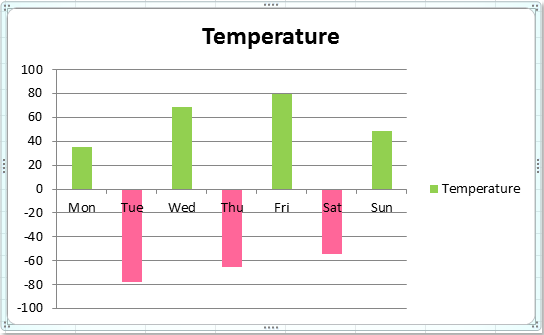
How to separate colors for positive and negative bars in column/bar chart?

Edit titles or data labels in a chart - support.microsoft.com To edit the contents of a title, click the chart or axis title that you want to change. To edit the contents of a data label, click two times on the data label that you want to change. The first click selects the data labels for the whole data series, and the second click selects the individual data label. Click again to place the title or data ...

Excel chart not printing correctly - i have a simple excel file (office

Chart: Display alternative values as Data Labels or Data Callouts Joined. Aug 11, 2017. Messages. 1. Aug 11, 2017. #1. Below is my excel chart. I would like to add a "data labels" or "data callouts". As you can see the line is displaying the data from Actual X and Y, but I want to display the DEV values on this line.

How to Create a Step Chart in Excel - Automate Excel

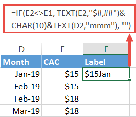
How to display different text than the value in same cell? 1. Select the cell values that you want to display them with different text, and then click Home > Conditional Formatting > New Rule, see screenshot: 2. Then in the New Formatting Rule dialog box, click Use a formula to determine which cells to format under the Select a Rule Type list box, and then enter this formula: =c1=1 ( C1 is the first ...

Enable or Disable Excel Data Labels at the click of a button - How To - PakAccountants.com

Custom data labels in a chart - Get Digital Help Press with mouse on "Add Data Labels". Press with mouse on Add Data Labels". Double press with left mouse button on any data label to expand the "Format Data Series" pane. Enable checkbox "Value from cells". A small dialog box prompts for a cell range containing the values you want to use a s data labels. Select the cell range and press with ...

Column Chart That Displays Percentage Change or Variance - Excel Campus

Combination Clustered and Stacked Column Chart in Excel Step 5 – Adjust the Series Overlap and Gap Width. In the chart, click the “Forecast” data series column. In the Format ribbon, click Format Selection.In the Series Options, adjust the Series Overlap and Gap Width sliders so that the “Forecast” data series does not overlap with the stacked column. In this example, I set both sliders to 0% which resulted in no overlap and a …

Scatter Plot Template in Excel | Scatter Plot Worksheet

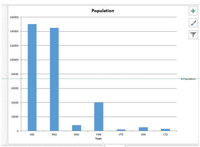
How to Add Axis Labels in Microsoft Excel - Appuals.com Click anywhere on the chart you want to add axis labels to. Click on the Chart Elements button (represented by a green + sign) next to the upper-right corner of the selected chart. Enable Axis Titles by checking the checkbox located directly beside the Axis Titles option. Once you do so, Excel will add labels for the primary horizontal and ...

ExcelMadeEasy: Vba charts in vba in Excel

How to Change Excel Chart Data Labels to Custom Values? First add data labels to the chart (Layout Ribbon > Data Labels) Define the new data label values in a bunch of cells, like this: Now, click on any data label. This will select "all" data labels. Now click once again. At this point excel will select only one data label. Go to Formula bar, press = and point to the cell where the data label ...

Format Data Labels in Excel- Instructions - TeachUcomp, Inc.

Two-Level Axis Labels (Microsoft Excel) Excel automatically recognizes that you have two rows being used for the X-axis labels, and formats the chart correctly. (See Figure 1.) Since the X-axis labels appear beneath the chart data, the order of the label rows is reversed—exactly as mentioned at the first of this tip. Figure 1. Two-level axis labels are created automatically by Excel.

Teach Besides Me: Data Labels Excel 2010

Design the layout and format of a PivotTable In a PivotTable that is based on data in an Excel worksheet or external data from a non-OLAP source data, you may want to add the same field more than once to the Values area so that you can display different calculations by using the Show Values As feature. For example, you may want to compare calculations side-by-side, such as gross and net profit margins, minimum and …

ChartSmartXL and Excel FAQs | Answers to Common Questions

How to show data labels in PowerPoint and place them ... - think-cell In think-cell, you can solve this problem by altering the magnitude of the labels without changing the data source. ×10 6 from the floating toolbar and the labels will show the appropriately scaled values. 6.5.5 Label content. Most labels have a label content control. Use the control to choose text fields with which to fill the label. For ...

Simple Bar Chart Beats Complex Multiple Sized Pies - Peltier Tech Blog

A Comprehensive Guide on Microsoft Excel for Data Analysis Nov 24, 2021 · You can make a chart, modify its type, adjust the row or column, the legend location, and the data labels. Column Chart, Line Chart, Pie Chart, Bar Chart, Area Chart, Scatter Plot are some of the different types of charts provided in Microsoft Excel. 10) Data Validation. Only valid values may need to be entered into cells.

Microsoft Office Excel 2010: A Lesson Approach, Complete 1st Edition Textbook Solutions | Chegg.com

Excel charts: add title, customize chart axis, legend and data labels ... Click anywhere within your Excel chart, then click the Chart Elements button and check the Axis Titles box. If you want to display the title only for one axis, either horizontal or vertical, click the arrow next to Axis Titles and clear one of the boxes: Click the axis title box on the chart, and type the text.

1. Introduction - Writing Excel Macros with VBA, 2nd Edition [Book]

Excel tutorial: How to customize axis labels Now let's customize the actual labels. Let's say we want to label these batches using the letters A though F. You won't find controls for overwriting text labels in the Format Task pane. Instead you'll need to open up the Select Data window. Here you'll see the horizontal axis labels listed on the right. Click the edit button to access the ...

Excel 2013: Label deconfliction in labeled scatter plot - Stack Overflow

3 Ways to Highlight Every Other Row in Excel - wikiHow Click and drag the mouse to select all the cells in the range you want to edit. If you want to highlight every other row in the entire document, press ⌘ Command + A on your keyboard. This will select all the cells in your spreadsheet. 3. Click the icon next to "Conditional Formatting."

Share :